The oscilloscope
See your signals in real time
An oscilloscope is an extremely useful piece of kit when working with electronics. Oscilloscopes allow you to visualise, examine and understand electronic signals varying in time. The Bela IDE includes an in-browser oscilloscope that you can use to display your signals in real time, right in your browser - no external tools required.
This article explains how to use the Bela oscilloscope.
Table of contents
- Visualising signals varying in time
- The basic principles of a scope
- Launching the Bela scope
- Basic controls
- Time vs Frequency domain
- Sending signals to the scope
Visualising signals varying in time
Oscilloscopes are devices that display the change in an electrical signal over time. As well as displaying signals continuously, oscilloscopes can also capture and display events that happen too fast to be seen as they unfold, in order to observe and understand them in non-realtime. Oscilloscopes are an essential tool for every electronic engineer, and every maker can benefit from understanding how to use them.
The basic principles of a scope
The basic principle of an oscilloscope is that you can view (scope) variations (oscillo) in an electrical signal over time. Analog oscilloscopes use a CRT display and have a characteristic greenish ray which is absolutely enchanting, but digital oscilloscopes are much more commonly used these days and come with quite a price tag.
On the display of an oscilloscope you will typically see a graph of the electronic signal where the x-axis represents time, and the y-axis represents voltage. Typically oscilloscope controls will allow you to change the scaling of the signal, as well as only refresh the plotting of a signal once it passes a certain threshold (known as triggering) so you can get a clear picture of a signal that might be moving too fast to see what’s really going on.
Launching the Bela scope
The scope can be launched by clicking the Scope button on the main toolbar. This will launch the scope in a new tab in your browser where you will see a visualisation of the signals that you are sending. If it’s your first time working with the scope we recommend launching the Fundamentals/scope example to see it in action.
The scope will be default show a signal that varies from 1.0 to -1.0 in your program although the scaling can be easily adjusted.
Basic controls
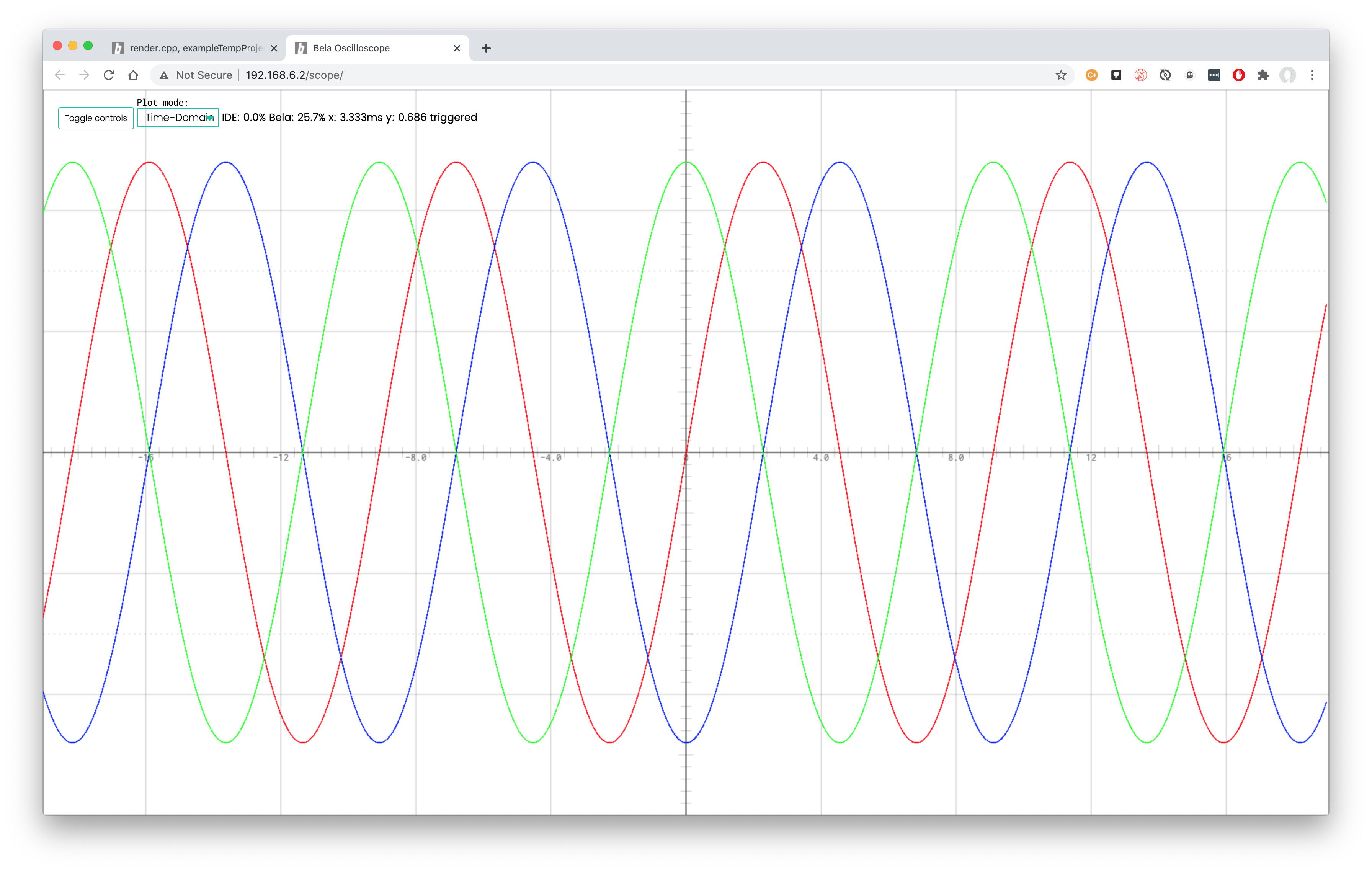
Once the scope has launched you should see the signal displayed in the window, in this case three sine waves out of phase from each other.
Click on the Toggle controls button in the top left corner to bring up the settings window.
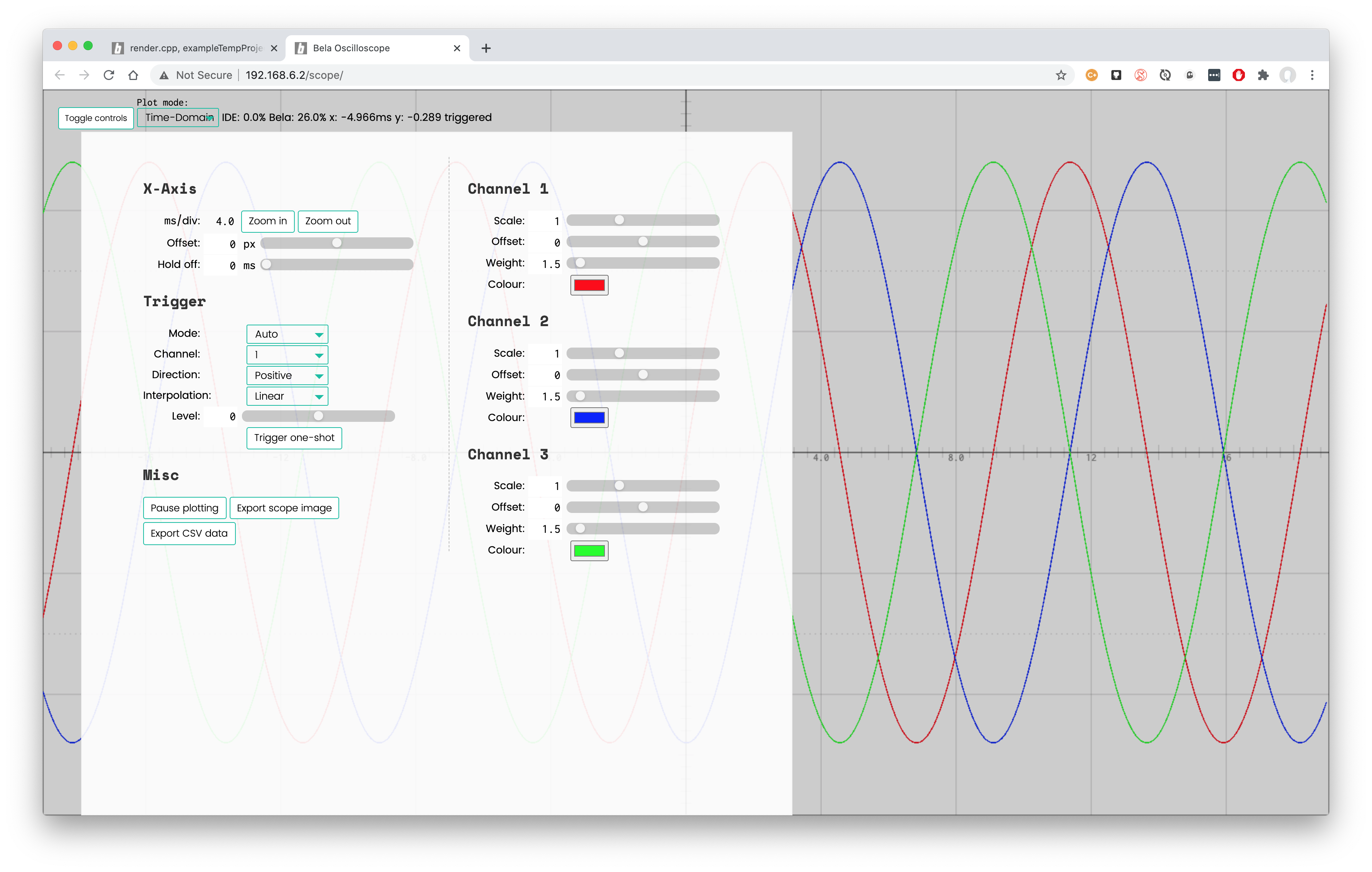
X-Axis
Here you can zoom in and out in time by setting the number of milliseconds which are shown per division of the screen (ms/div). You can also adjust the Offset of the whole x-axis and adjust the amount of time that a signal stays on the screen before refreshing with the Hold on setting.
Channel settings
The number of channels you see here will depend on the amount of channels you have set up in your code. There is no upper limit to the amount of channels that you can scope simultaneously (note that you are limited to 4 channels in Pure Data). For each channel you can customise the overall Scale, the Offset, the line Weight and the Colour.
Triggering
By default the oscilloscope will be in Auto trigger mode which mean that it refreshes the screen automatically and continues to show you the signal over time. We can also set the scope to freeze the image based on a certain trigger condition.
When set to Normal the scope will freeze it’s image when the signal on a selected Channel passes over a set threshold Level in either a positive or negative Direction. This is very useful for freezing the image of the scope when a sensor reading goes high: for example if you are looking at triggering events based on the signal from a piezo disk or force sensitive resistor.
When the trigger mode is set to Custom you can send a message from your code to freeze the scope images at any arbitrary moment in time. This is extremely useful for debugging hardware that requires precise timing, or simply for visualising various states in your software. Remember that you can visualise any signal in your program, not just the audio and sensor signals.
Miscellaneous controls
It is also possible manually pause the plotting of the scope with the button Pause plotting.
You can export the data captured on the scope in a couple of ways: Export CSV data give you the data for further analysis; Export scope image will generate a .png image of the current plot.
Time vs Frequency domain
As well as viewing signals in the time domain, you can also switch the scope into the frequency domain via the FFT button on the top left hand side. Looking at the signal in the frequency domain means that we will be able to see how the different frequencies present in the signal vary in time.
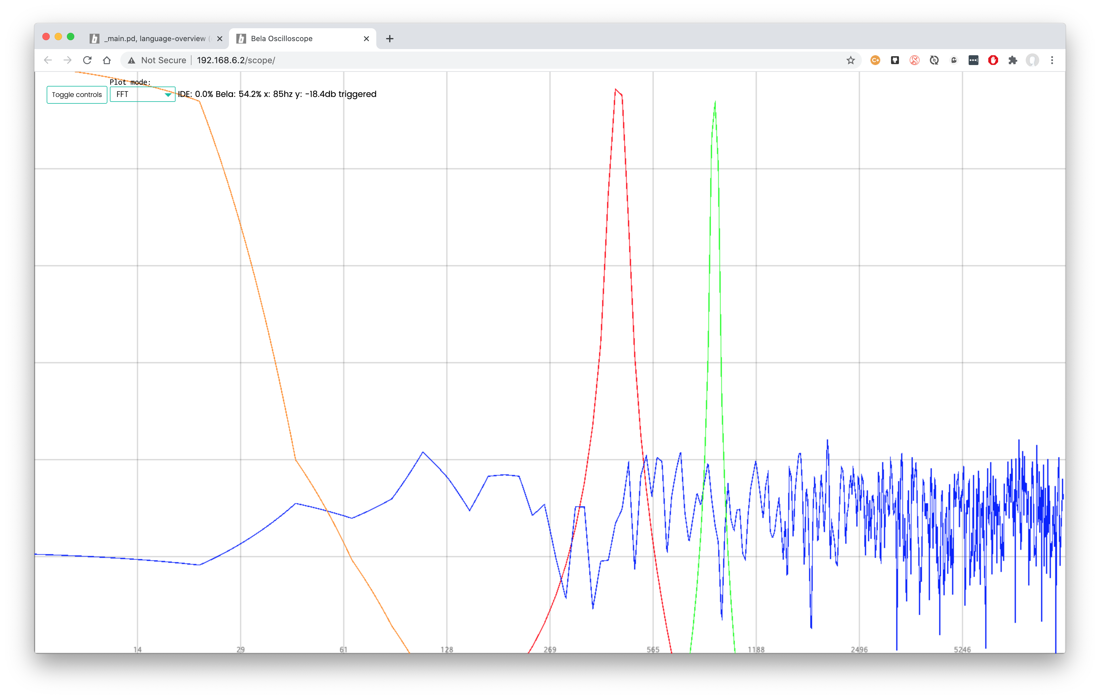
In FFT mode we’ll also get some new settings. The FFT Length is an import setting to experiment with. If you set this to be a lower value you will get better temporal definition but worse frequency definition. Contrastingly if you set the FFT length to be a higher value you will get better frequency definition and worse temporal definition.
You can also change whether the y-axis is displayed as Normalised or Decibel scale better for seeing the loudness of audio signals. Equally you can switch the x-axis scaling from Linear to Logarithmic which is better for viewing musical pitch relationships.
Sending signals to the scope
To understand how to send signals to the oscilloscope the best thing to do is look at the example for the specific programming language you are using.
- For projects in c++ have a look at the following examples: Fundamentals/scope; Fundamentals/scope-advanced; Analog/scope-analog.
- For projects in Pure Data have a look at the following examples: PureData/language-overview; PureData/oscilloscope.
- For projects in SuperCollider have a look at the following example: SuperCollider/8-scope.