Oscilloscope
Visualising sensor signals and audio
The Bela IDE includes a built-in oscilloscope, an extremely useful debugging tool. In this tutorial we’ll hook up two analog potentiometers and use them to explore some of the oscilloscope’s functionality, examining both the time and frequency domain.
Table of contents
The toolbox of an electronic engineer
Oscilloscopes are an essential tool for every electronic engineer, and every maker can benefit from understanding how to use them.
The basic principle of an oscilloscope is that you can view (scope) variations (oscillo) in an electrical signal over time. Analog oscilloscopes use a CRT display and have a characteristic greenish ray, but digital oscilloscopes are much more commonly used and visualise signals on a monitor.
An oscilloscope allows you to graph electronic signals as they vary in time. On the display of an oscilloscope you will typically see a graph of the signal where the x-axis represents time, and the y-axis represents voltage. Typically oscilloscope controls will allow you to change the scaling of the signal, as well as freeze an image of the signal once it passes a certain threshold (known as triggering) so you can get a clear picture of a signal that might be moving too fast to see what’s really going on. e signals our sensors produce.
Hardware setup
For this project we need to connect a force sensing resistor (also know as a pressure sensor or FSR) to analog input 0 and a potentiometer (also know as a dial) to analog input 1. Both of these sensors work by varying their resistance.
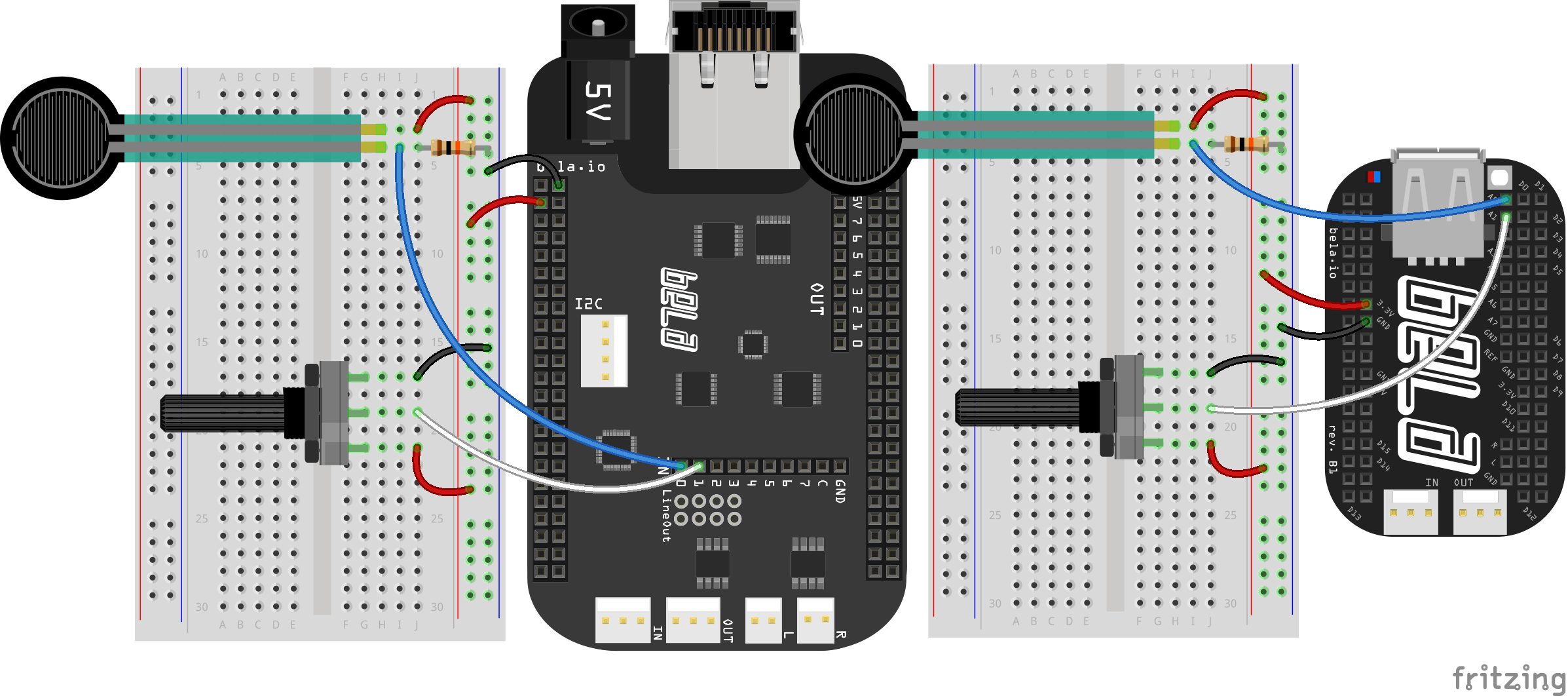
First note that the potentiometer has three pins, let’s call them Ground, Signal and Power going from left to right. By turning the dial we change the amount of resistance on either side of the central Signal pin of the potentiometer. This changes the relative “closeness” of that pin to Power or Ground, giving us a different voltage which we can read with analog input of Bela. The FSR functions in a similar manner but with a fixed value resistor on one side.
The code
Find the oscilloscope sketch in the Pure Data section of the Examples tab of the Bela IDE.
1. Sending signals to the scope
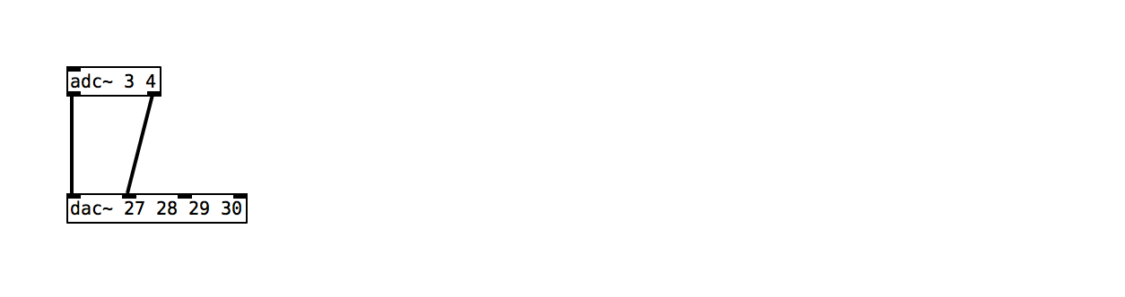
You can log any signal to the scope by connecting it to [dac~ 27 28 29 30]. Just as we saw for the analog outputs we use a special range of channels on the [dac~] object, in this case channels 27-30.
We can send anything we want to the scope whether sensor signal or audio signal but we need to make sure the signal is at audio rate which in Pure Data means that the object must have a ~. To convert a control rate signal to audio rate you can use the [sig~] object.
2. Filtered noise
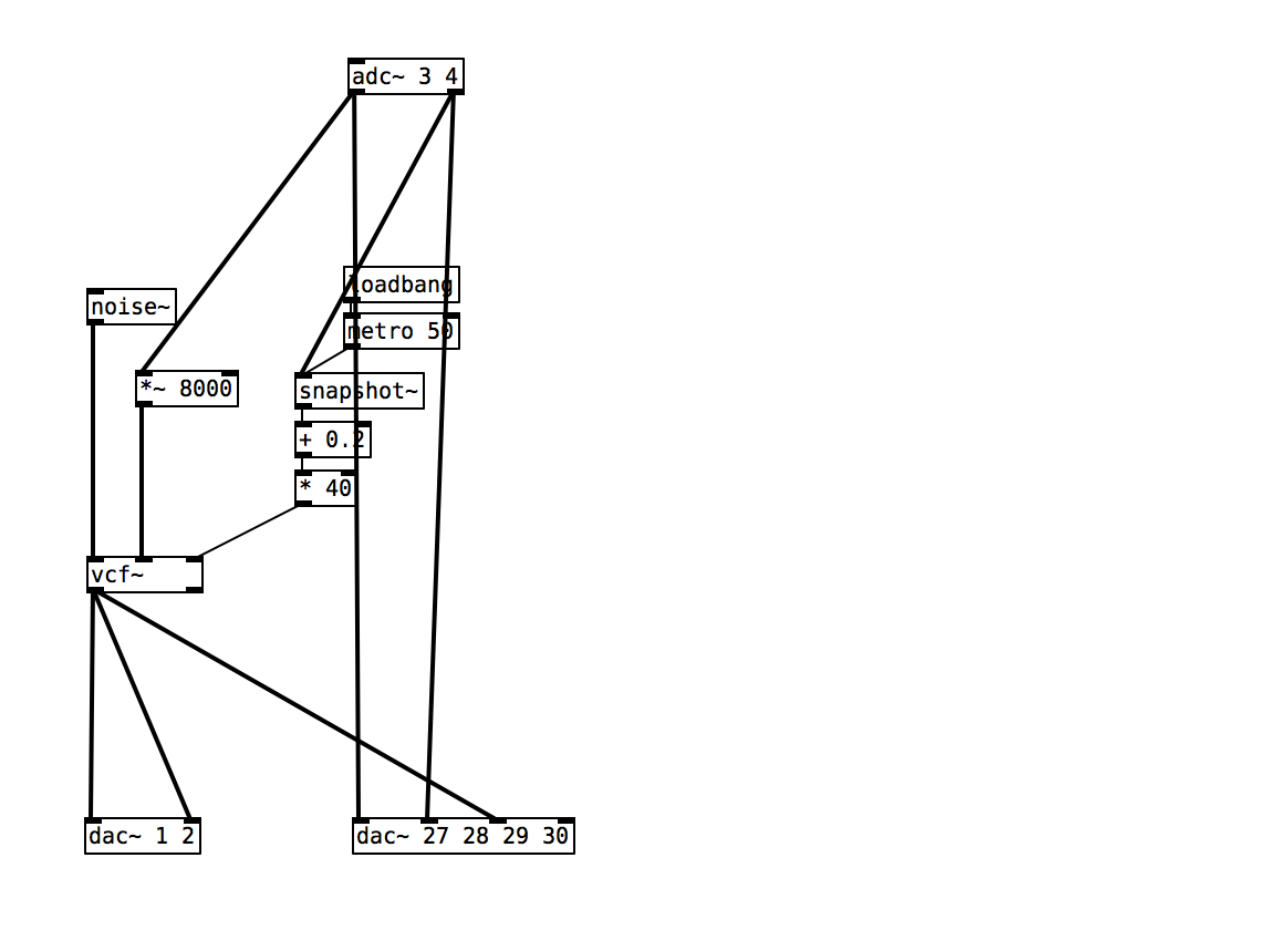
The rest of this patch controls a bandpass filter which has a white noise source fed into it. Bandpass filters allow a certain frequency band to pass through them, while rejecting all other frequencies.
Practice tasks
Task 1: Look at sensor signals on the scope
We have the first two analog inputs connected to the first two channels of the oscilloscope on [dac~ 27 28]. To view the signals launch the scope in IDE by pushing the scope button. Try moving the potentiometers and watch the effect on the scope.
Task 2: Trigger the scope from the FSR signal
As well as viewing the signals from the sensors continuously in time it is also possible to take a snapshot of the signal which will be paused in time so you can have a good look. To do this first click the Toggle controls button to bring up the control panel. The default mode, where the screen is constantly refreshing is Auto mode. To set things into trigger mode change the Mode: setting to Normal.
When the scope is set into Normal mode it will wait for a signal to pass over a certain threshold before taking a snapshot of that signal. Looking at the Trigger settings we can see that we can choose the channel which should be monitored for the trigger, the direction in which the signal should pass the threshold (either from below or from above), the interpolation of the signal which smooths out fluctuations, and most importantly the threshold level.
Try setting the threshold level to around 0.4 and then tapping on the FSR. When you tap on the FSR you will see a sudden increase in the signal on the scope. This is what we are using to trigger the snapshot. Try tapping multiple times and also zooming out to look at the changes in the signal over a longer time period.
Task 3: Switch the scope into the frequency spectrum
So far we have been using the scope in the time domain, looking at how the voltages received in the analog inputs vary over time. Now let's connect the output of the filter to the third input of the scope and open the scope. We can see the waveform of the audio signal which changes constantly and waves get larger or smaller depending on how we move the potentiometer.
We can also look at this signal in the frequency domain meaning that we will be able to see how the different frequencies present in the signal vary in time. To do this we switch the scope into FFT mode in the top left.
Try adjusting the various setting you have in the control panel to see the signal better. If you set the window size to be a lower value you will get better temporal definition but worse frequency definition. Contrastingly if you set the window size to be a higher value you will get better frequency definition and worse temporal definition. Try also putting the scope into decibel mode and zooming in on the frequency range (x axis).
If you move the pots you will see the frequency spike moving on the x axis and growing on the y axis. This is because we are controlling the cutoff frequency and Q of the filter.
Task 4: Look at the different effects of a bandpass and low pass filter.
The [vcf~] object can give you both a bandpass filter and lowpass filter depending on which outlet you use. Try connecting both of these outlets to the scope to compare the spectrums of both. This should help you understand the effects of both these filter types.